Virtual Laboratory

Virtual Labs are intended to augment the learning of engineering subjects through performing experiments. The experiments are designed either as simulations or as remote triggered. A remote triggered lab allows a user to connect to real equipments using web browser.

Key Features:

  • Includes VTU EC-DSP Laboratory experiments of CBCS-2018/2021/2022 Scheme.
  • Machine Learning Classifiers designed for handling data.
  • ML-Classifiers furnishes details like Confusion Matrix,Classification report, Actual vs Predicted data labels and Accuracy for the testing dataset.
  • Includes VTU EC Advance communication Laboratory experiments of CBCS-2018/2021/2022 Scheme.
  • Includes VTU EC Analog/Digital simulation experiments of CBCS-2018/2021/2022 Scheme.
  • Circuit simulation animator with demonstration video.

Click here to download programs related to single/multiple table.

About Us

Department of Electronics and Communication Engineering, Vivekananda College of Engineering and Technology, Puttur

Electronics and Communication Engineering is a 4-year degree programme, affiliated to the VTU was started in the year 2001. ECE is the utilization of science and math applied to practical problems in the field of communications. It includes designing, fabrication, testing, maintenance, supervision, and manufacturing of electronic equipments in entertainment, media, hospitals (Medical Electronics), computer control systems, broadcast, communication systems and in defence. It also engage in research, design, development and testing of electronic equipment used in various communication systems. The defined courses aim to prepare students to play a leading role in the continuing adventure of modern communication, research, designing, building and marketing the next generation of products.

Convolution

Inputs
Example:1 2 3
Example:1 2 3
Example for Linear Convolution
∑      x(k)h(n-k)=y(n)
k=-∞
Eg: let x(n)={1,2,3} and h(n)={1,1,1}

y(0)=∑x(k)h(-k)=x(0)h(0)=1
y(1)=∑x(k)h(1-k)=x(0)h(1)+x(1)h(0)=3
y(2)=∑x(k)h(2-k)=x(0)h(2)+x(1)h(1)+x(2)h(0)=6
y(3)=∑x(k)h(3-k)=x(1)h(2)+x(2)h(1)=5
y(4)=∑x(k)h(4-k)=x(2)h(0)=3

Example for Circular Convolution
N-1
∑      x(k)h((n-k))N=y(n)
k=0
Eg: let x(n)={1,2,3} and h(n)={1,1,1}

y(0)=∑x(k)h((-k))3=x(0)h(0)+x(1)h((-1))3+x(2)h((-2))3=6
y(1)=∑x(k)h((1-k))3=x(0)h(1)+x(1)h((0))3+x(2)h((-1))3=6
y(2)=∑x(k)h((2-k))3=x(0)h(2)+x(1)h((1))3+x(2)h((0))3=6

Correlation

Inputs
Example:1 2 3
Example:1 2 3
Equation with Example
∑   x(k)h(k-n)=y(n)
k=-∞
Eg: let x(n)={1,2,3} and h(n)={3,2,1}

y(0)=∑x(k)h(k)=x(0)h(0)+x(1)h(1)+x(2)h(2)=10
y(1)=∑x(k)h(k-1)=x(1)h(0)+x(2)h(1)=12
y(2)=∑x(k)h(k-2)=x(2)h(0)=9
y(-1)=∑x(k)h(k+1)=x(0)h(1)+x(1)h(2)=8
y(-2)=∑x(k)h(k+2)=x(0)h(2)=1

FFT

Inputs
Example:1 2 3 4
Equation with Example
N-1
∑     x(n)e-j2Πkn/N=X(k)
n=0
Eg: let x(n)={1,2,3,4}

X(0)= x(0)e0+x(1)e0+x(2)e0+x(3)e0=10
X(1)= x(0)e0+x(1)e-j2Π/4+x(2)e-j4Π/4+x(3)e-j6Π/4=-2+2j
X(2)= x(0)e0+x(1)e-j4Π/4+x(2)e-j8Π/4+x(3)e-j12Π/4=-2
X(3)= x(0)e0+x(1)e-j6Π/4+x(2)e-j12Π/4+x(3)e-j18Π/4=-2-2j

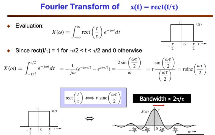
Fourier Transform of Rectangular Pulse

Inputs
Example:1
Example:1
Example:100
Equation with Example. Click here for better image quality.

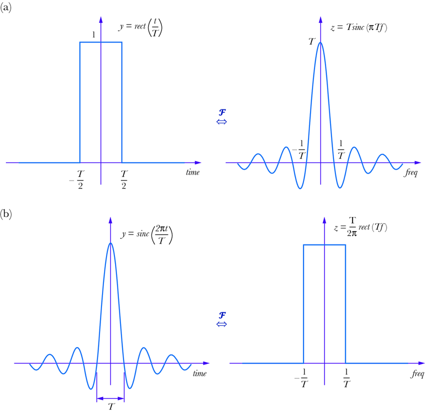
Fourier Transform of Sinc Pulse

Inputs
Example:1
Example:1
Example:100
Equation with Example. Click here for better image quality.

DCT

Inputs
Example:1 2 3
Equation with Example
N-1
∑     x(n)cos(Π(2n+1)k/2N)*w(k)=X(k)
n=0

With w(0)=sqrt(1/N) and w(k)=sqrt(2/N), for k=1,2..N-1

Eg: let x(n)={1,2,3}

X(0)= (x(0)cos(0)+x(1)cos(0)+x(2))*sqrt(1/3)=3.464
X(1)= (x(0)cos(Π/6)+x(1)cos(3Π/6)+x(2)cos(5Π/6))*sqrt(2/3)=-1.414
X(2)= (x(0)cos(2Π/6)+x(1)cos(6Π/6)+x(2)cos(10Π/6))*sqrt(2/3)=0

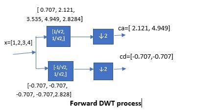
DWT

Inputs
Example:1 2 3 4
Example:0.7071 0.7071
Example:-0.7071 0.7071
DWT process

MFCC

Inputs
Example:512
Example:0.5
Example:20
MFCC algorithm usage guidelines
1. Provide .wav file only.
2. wav sample files are available for download here.
3. These algorithm returns Original speech signal and MFCC features.
4. The dimension of MFCC features depends on filter bank size, provided by the user.
5. Data furnished by these algorithm may used in Speech recognization system for validation

FIR Filter

Inputs
Example:21
Example:0.785
Example:hamm/hann
Low pass FIR filter analysis
hd(n)= 1/2 -wcwc e-jwαejwndw

hd(n)= sin(wc(n-α))/(Π(n-α))

h(n)= hd(n)w(n), 0<=n<=N-1

H(w)= ∑h(n)e-jwn

Difference Equation

Inputs
Example:1 2
Example:1 -4 3
Example:1 2 3 4
Difference equation
y(n)= - ∑k=0N aky(n-k)+∑k=0M bkx(n-k)
Eg: let x(n)={1,2,3,4}, b0=1,b1=2, a1=-4,a2=3

y(n)=-a1y(n-1)-a2y(n-2)+b0x(n)+b1x(n-1)+b2x(n-2)
y(0)=4y(-1)-3y(-2)+x(0)+2x(-1)=1
y(1)=4y(0)-3y(-1)+x(1)+2x(0)=8
y(2)=4y(1)-3y(0)+x(2)+2x(1)=36
y(3)=4y(2)-3y(1)+x(3)+2x(2)=130

IIR filter

Inputs
Example:1500
Example:3000
Example:3
Example:10
Example:8000
Design procedure
Eg: Let Fp=1500Hz, Fs=3000Hz, ap=3dB, as=10dB, Fsamp=8000Hz, T=1/Fsamp ωp=2πFp/Fsamp=0.375π, ωs=2πFs/Fsamp=0.75π Ωp=(2/T)tan(ωp/2)=1.069x104,Ωs=(2/T)tan(ωs/2)=3.862x104
  • Obtain order N= log(10(ap/10) -1/10(as/10) -1)/(2log(Ωp/Ωs)~=1
  • Obtain ωc=ωp=0.375π
  • Obtain Han(s) = 1/(s+1)
  • Obtain HLp(s) = Han(s)|s->s/Ωp= (1.069x10⁴)/(s+1.069x104)
  • Obtain H(z)=HLp(s)|z->(2/T)(1-z-1)/(1+z-1)=(0.4006+0.4006z-1)/(1-0.1977z-1)
  • Obtain H(w)= H(z)|z->ejw

Sampling Theorem

Inputs
Example:10
Example:100
Example:0.0001
Sampling theorem statement and cases
Sampling theorem statement : A signal x(t) can be reconstructed successfully from its samples x(n) if fs>=2fm
Three cases of sampling theorem
  • Case(i) Oversampling: fs>>2fm, reconstruction is possible, but not effective since it consumes more memory
  • Case(ii)Nyquist rate sampling: fs=2fm,reconstruction is possible, effective since it does not consume more memory
  • Case(iii)Under sampling: fs<<2fm,reconstruction is not possible

Overlap Save method

Inputs
Example:1 -1 1 2 -1 0 1 2 1
Example:1 -1 1
Example:5
Overlap save algorithm

Given the values of x(n), h(n) and length of block size N.
Overlap save method uses following steps to obtain the response y(n).
Step 1: Padd L-1 zeros to h(n) to make its length N. Where N=L+M-1 and M is length of h(n)
Step 2: Decompose x(n) into x1(n), x2(n), x3(n) and so on. To obtain x1(n), we padd (M-1) zeros at the beginning and extract first L samples of x(n). Similarly x2(n) is obtained by considering the last (M-1) samples of x1(n) and next L samples of x(n). These process is repeated untill we visit all samples of x(n).
Step 3: Find the circular convolution between x1(n) and h(n), indicate it by y1(n)
Step 4: Repeat step 3 to obtain y2(n), y3(n) and so on.
Step 5: Discard the first (M-1) samples of each output sequences, remaining samples are fitted one after another to get the final sequence.

Overlap add method

Inputs
Example:1 -1 1 2 -1 0 1 2 1
Example:1 -1 1
Example:5
Overlap add algorithm

Given the values of x(n), h(n) and length of block size N.
Overlap save method uses following steps to obtain the response y(n).
Step 1: Padd L-1 zeros to h(n) to make its length N. Where N=L+M-1 and M is length of h(n)
Step 2: Decompose x(n) into x1(n), x2(n), x3(n) and so on. To obtain x1(n), we extract first L samples of x(n) and padd (M-1) zeros at the end. Similarly x2(n) is obtained by considering the next L samples of x(n) and padding (M-1) zeros at the end. These process is repeated untill we visit all samples of x(n).
Step 3: Find the circular convolution between x1(n) and h(n), indicate it by y1(n)
Step 4: Repeat step 3 to obtain y2(n), y3(n) and so on.
Step 5: Add the last (M-1) samples of each output sequences with the first (M-1) samples of succeedding output sequences, remaining samples are fitted one after another to get the final sequence.

Radix-2 DIT FFT

Inputs
Example:1 1 1 1 0 0 0 0
Radix-2 DIT FFT Algorithm for N=8

In Radix-2 DIT FFT algorithm, the input sequence x(n) is decimated in time domain. The decimation process is repeated untill x(n) becomes a 2 point sequence. Radix-2 is a process in which N point DFT's are represented using several two point DFT's.

Inverse Radix-2 DIT FFT

Inputs
Example:4 1 0 1 0 1 0 1
Example:0 -2.41421 0 -0.41421 0 0.41421 0 2.41421
Inverse Radix-2 DIT FFT Algorithm for N=8

In Inverse Radix-2 DIT FFT algorithm, the output sequence x(n) is decimated in time domain. The decimation process is repeated untill x(n) becomes a 2 point sequence. Radix-2 is a process in which N point IDFT's are represented using several two point IDFT's.

Radix-2 DIF FFT

Inputs
Example:1 1 1 1 0 0 0 0
Radix-2 DIF FFT algorithm

In Radix-2 DIF FFT algorithm, the input sequence x(n) is taken in natural order. The output sequence X(k) is taken in bit-reversed order. Radix-2 is a process in which N point DFT's are represented using several two point DFT's.

ASK Modulation

Inputs
Example:1000
Example:100
Example:0.1
Example:1
Amplitude Shift Keying theory
1. In ASK, the amplitude of the carrier signal is varied in accordance with the message signal
2. Carrier is transmitted if message bit is 1, is blocked if message bit is 0.
3. Also known as ON-OFF keying

FSK Modulation

Inputs
Example:1000
Example:50
Example:20
Example:0.1
Example:1
Frequency Shift Keying theory
1. In FSK, the frequency of the carrier signal is varied in accordance with the message signal
2. In FSK two carrier frequency are to be selected for bi1-1 and bit-0 respectively
3. Carrier frequency Fc1 is transmitted if message bit is 1.
4. Carrier frequecny Fc2 is transmitted if message bit is 0.

PSK Modulation

Inputs
Example:1000
Example:20
Example:0.1
Example:1
Phase Shift Keying theory
1. In PSK, the phase of the carrier signal is varied in accordance with the message signal
2. Carrier with no phase-shift is transmitted if message bit is 1.
3. Carrier with 180 degree phase-shift is transmitted if message bit is 0.

DPSK Modulation

Inputs
Example:1000
Example:20
Example:0.1
Example:1
Example:1/0
Differential Phase Shift Keying theory
1. In DPSK, the phase of the carrier signal is varied in accordance with the message signal
2. The message signal is differentially encoded(EXNOR) using initial bit d as 1 or 0.
3. Carrier with no phase-shift is transmitted if message bit is 1.
4. Carrier with 180 degree phase-shift is transmitted if message bit is 0.

QPSK Modulation

Inputs
Example:1000
Example:20
Example:0.1
Example:1
Quadrature Phase Shift Keying theory
1. In QPSK, the phase of the carrier signal is varied in accordance with the message signal
2. Here instead of single bit, di-bits are considered for modulation.
3. If message bit is 00, Carrier with 135 degree phase-shift is transmitted.
4. If message bit is 10, Carrier with 45 degree phase-shift is transmitted.
5. If message bit is 11, Carrier with 315 degree phase-shift is transmitted.
6. If message bit is 01, Carrier with 225 degree phase-shift is transmitted.

QAM Modulation

Inputs
Example:1000
Example:20
Example:0.1
Example:1
Quadrature Amplitude Modulation
1. In QAM, the amplitude and phase of the carrier signal is varied in accordance with the message signal
2. Here instead of single bit, four(quad)bits are considered for modulation.
3. Using quad bits, we get 16 possible combination with varied amplitude and phase.

TDM Modulation

Inputs
Example:1000
Example:5
Example:20
Example:0.01
Example:1
TDM Modulation
1. In TDM, two or more signals are multiplexed in time based on the control signal.
2. If number of message signals to be multiplexed is restricted to two and control signal is high, first message signal is transmitted.
3. If control signal is low, second message signal is transmitted.

Find-S

Inputs
Find-S Algorithm usage guidelines
1. Provide .csv file only.
2. Last column of the CSV file should have Yes or No labels.
3. CSV sample files are available for download here.

Decision Tree-ID3

Inputs
ID3 Algorithm usage guidelines
1. Provide .csv file only.
2. Last column of the CSV file should have Yes or No labels.
3. CSV sample files are available for download here.

Candidate-Elimination Algorithm

Inputs
Candidate-Elimination Algorithm usage guidelines
1. Provide .csv file only.
2. Last column of the CSV file should have Yes or No labels.
3. CSV sample files are available for download here.

Logistic Regression

Inputs
Example:0.25
Logistic Regression Classifier usage guidelines
1. Provide .csv file only.
2. Remove column and row names from the csv file if existing.
3. Last column of the CSV file should have class label in integer form.
4. CSV sample files are available for download here.

KNN Classifier

Inputs
Example:5
Example:0.25
KNN Classifier usage guidelines
1. Provide .csv file only.
2. Remove column and row names from the csv file if existing.
3. Last column of the CSV file should have class label in integer form.
4. Number of neighors should be entered.
5. CSV sample files are available for download here.

Random Forest

Inputs
Example:0.25
Random Forest Classifier usage guidelines
1. Provide .csv file only.
2. Remove column and row names from the csv file if existing.
3. Last column of the CSV file should have class label in integer form.
4. Max depth parameter for Classifier is set to 2.
5. CSV sample files are available for download here.

Linear Discriminant Classifier

Inputs
Example:0.25
Linear Discriminant Analysis(LDA) Classifier usage guidelines
1. Provide .csv file only.
2. Remove column and row names from the csv file if existing.
3. Last column of the CSV file should have class label in integer form.
4. No. of components for classifier is to default= min(no of features,no of classes-1).
5. CSV sample files are available for download here.

Decision Tree

Inputs
Example:0.25
Decision Tree Classifier usage guidelines
1. Provide .csv file only.
2. Remove column and row names from the csv file if existing.
3. Last column of the CSV file should have class label in integer form.
4. Max depth parameter for Classifier is set to 2.
5. CSV sample files are available for download here.

Linear Support Vector Machine

Inputs
Example:0.25
Linear SVM Classifier usage guidelines
1. Provide .csv file only.
2. Remove column and row names from the csv file if existing.
3. Last column of the CSV file should have class label in integer form.
4. Linear Kernel is selected.
5. CSV sample files are available for download here.

Non Linear Support Vector Machine

Inputs
Example:0.25
Non Linear SVM Classifier usage guidelines
1. Provide .csv file only.
2. Remove column and row names from the csv file if existing.
3. Last column of the CSV file should have class label in integer form.
4. RBF Kernel is selected.
5. CSV sample files are available for download here.

Circuits Lab

Circuits Lab Videos

Op-Amp Inverting Amplifier

Half Adder

Half Wave Rectifier

Contact

Department of Electronics and Comunication Engineering, Vivekananda College of Engineering and Technology Puttur

Location:

Neharunagara, Puttur, D. K. Karnataka

Call:+91 9743703473